Getting started with dynR

What is dynamic functional connectivity?

Resting-state fMRI measures the BOLD signal across brain regions over time. Static functional connectivity (FC) compresses this into a single correlation matrix — the time-averaged co-activation pattern across the entire scan. Convenient, but it discards everything that changes.

Dynamic functional connectivity (dynFC) treats the time dimension seriously. It asks: does the pattern of co-activation between brain regions shift during a scan, and can those shifts tell us something about cognition, clinical state, or neural mechanisms?

dynR computes dynFC representations from preprocessed multivariate timeseries, implementing two complementary families of methods:

Family	Core functions	What it captures
Phase-based	`hilbert_phases()`, `dyn_phase_lock()`, `kuramoto()`	Instantaneous synchrony via the analytic signal
Correlation-based	`corr_slide()`, `cofluct()`, `corr_corr()`	Windowed co-activation and edge dynamics

Both families produce outputs that feed directly into stateR for brain state quantification.

When to use which approach

Choosing between phase-based and correlation-based methods depends on your research question:

	Phase-based	Correlation-based
Temporal resolution	Frame-by-frame (no window needed)	One estimate per window
Feature dimensionality	N (one eigenvector per timepoint)	N(N−1)/2 (upper triangle)
Window length choice	Not required	Critical parameter
Best for	Synchrony research, tractable state clustering, metastability	Interpretable FC, task-event alignment, edge dynamics

If you are new to dynFC, the phase-based / LEiDA pipeline is a good starting point: it requires no window length decision and produces compact, interpretable features. Sliding-window FC is more directly comparable to the broader published literature and easier to relate to task structure or behavioural events.

Package data

dynR ships with a resting-state BOLD fMRI timeseries from the edge-ts repository (Faskowitz et al., 2020), parcellated into 200 regions of interest. This dataset is used throughout all three vignettes. The methods themselves are not restricted to fMRI — they apply equally to EEG, LFP, or any band-limited neurophysiological signal.

data(ts)   # [200 × 600] BOLD timeseries
data(fc)   # [200 × 200] static FC matrix (ground truth)

dim(ts)
#> [1] 200 600
dim(fc)
#> [1] 200 200

200 parcels, 600 timepoints — approximately 20 minutes at TR = 2 s.

Pipeline overview

BOLD timeseries [N × Tmax]
        │
        ├─── bandpass_filter()       optional: restrict to 0.01–0.1 Hz
        │
        ├─── PHASE-BASED ─────────────────────────────────────────────
        │     hilbert_phases()   →  instantaneous phases  [N × Tmax]
        │     dyn_phase_lock()   →  dPL matrices + LEiDA eigenvectors
        │     kuramoto()         →  synchrony, metastability, entropy
        │
        └─── CORRELATION-BASED ───────────────────────────────────────
              corr_slide()      →  FC matrices  [N × N × windows]
              cofluct()         →  edge time series + RSS
              corr_corr()       →  FC recurrence  [Tmax × Tmax]
                    │
                    ▼
              stateR  ──  fractional occupancy
                      ──  dwell time
                      ──  Markov transitions

Quick example: phase-based pipeline

# Instantaneous phases via the Hilbert transform
phases <- hilbert_phases(ts)

# Dynamic phase-locking matrices + LEiDA eigenvectors
dpl <- dyn_phase_lock(phases)
cat("LEiDA matrix:", nrow(dpl$leida), "timepoints ×",
    ncol(dpl$leida), "parcels\n")
#> LEiDA matrix: 580 timepoints × 200 parcels

# Kuramoto order parameter
kop <- kuramoto(phases)
cat("Metastability:", round(kop$metastability, 4), "\n")
#> Metastability: 0.0796

ggplot(data.frame(t = seq_along(kop$synchrony), R = kop$synchrony),
       aes(x = t, y = R)) +
  geom_line(colour = "#8D9FD7", linewidth = 0.7) +
  geom_hline(yintercept = mean(kop$synchrony),
             colour = "#9E3C30", linetype = "dashed", linewidth = 0.9) +
  scale_y_continuous(limits = c(0, 1)) +
  labs(x = "Timepoint", y = "R(t)",
       title = "Kuramoto order parameter",
       subtitle = paste0("Metastability = ",
                         round(kop$metastability, 4))) +
  theme_minimal(base_size = 13) +
  theme(panel.grid.minor = element_blank())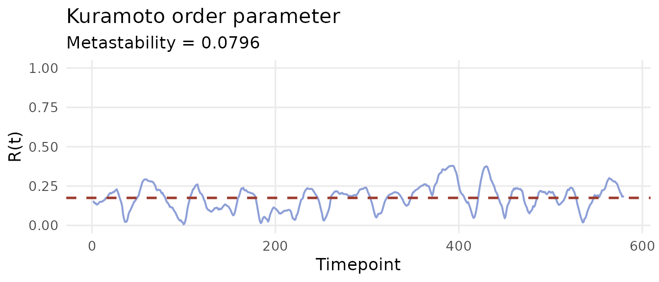

Quick example: correlation-based pipeline

# Sliding-window FC: 30-timepoint windows, step 5
sw <- corr_slide(ts, window = 30, step = 5)
cat("Windows:", dim(sw$corr_mats)[3], "\n")
#> Windows: 115

# Edge-centric cofluctuations
ec <- cofluct(ts)
cat("Edges:", nrow(ec$edge_ts), "× Timepoints:", ncol(ec$edge_ts), "\n")
#> Edges: 19900 × Timepoints: 600

ggplot(data.frame(t = seq_along(ec$rss), rss = ec$rss),
       aes(x = t, y = rss)) +
  geom_line(colour = "#8D9FD7", linewidth = 0.7) +
  geom_hline(yintercept = mean(ec$rss) + 2 * sd(ec$rss),
             colour = "#9E3C30", linetype = "dashed", linewidth = 0.9) +
  labs(x = "Timepoint", y = "RSS",
       title = "Root-sum-square cofluctuation",
       subtitle = "Dashed line: mean + 2 SD") +
  theme_minimal(base_size = 13) +
  theme(panel.grid.minor = element_blank())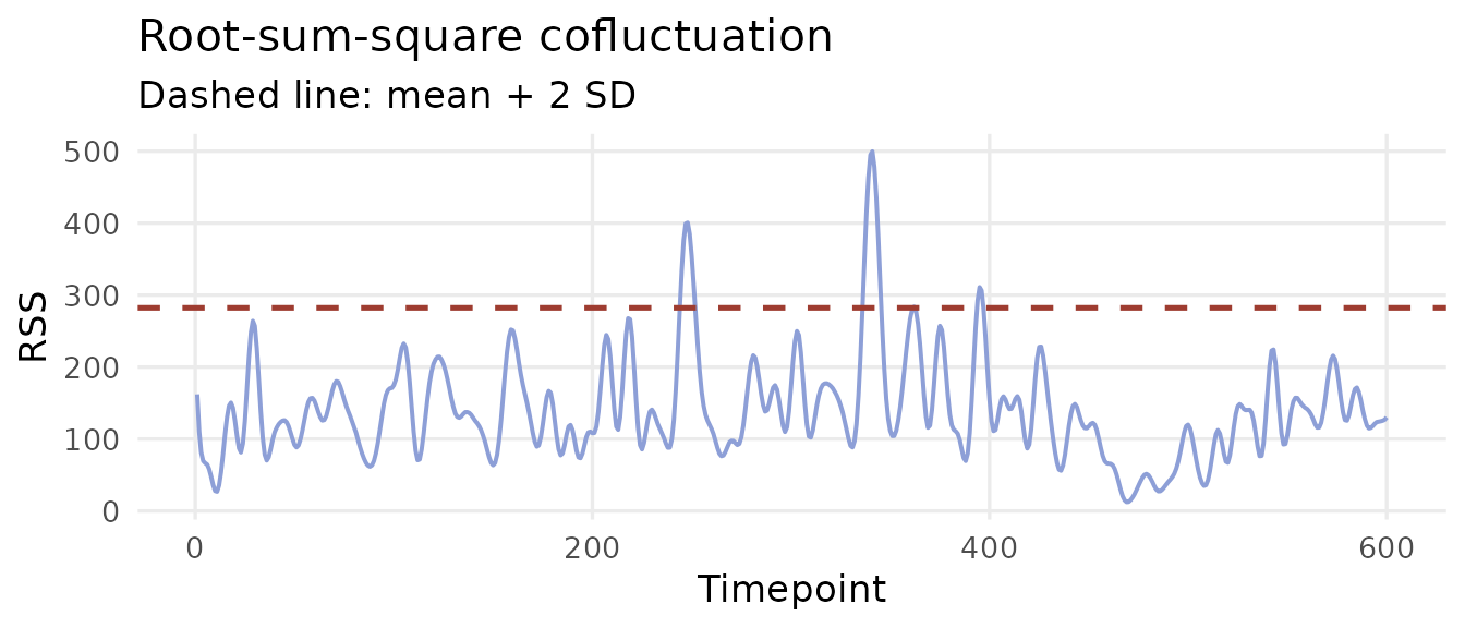

Sanity check: single window equals static FC

A single window spanning the full timeseries must recover the static FC matrix exactly — a useful first validation for any new dataset.

full_window <- corr_slide(ts, window = ncol(ts))
max_diff    <- max(abs(full_window$corr_mats[, , 1] - fc))
cat("Max deviation from static FC:", formatC(max_diff, format = "e"), "\n")
#> Max deviation from static FC: 8.8818e-16

References

Faskowitz, J. et al. (2020). Edge-centric functional network representations of human cerebral cortex reveal overlapping system-level architecture. Nature Neuroscience, 23(12), 1644–1654. https://doi.org/10.1038/s41593-020-00719-y